
 |
 |
 |
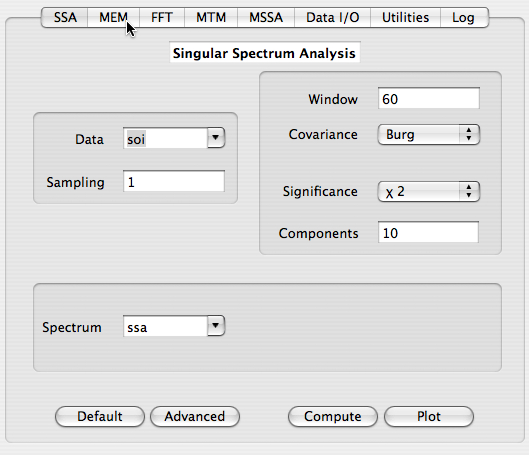
Having selected the data vector to be analyzed (here `soi', the SOI time-series), and the value of sampling interval, the main SSA options to be specified are the Window Length, the type of Significance
, and Covariance Estimator. The Default button is provided as a guide to select input parameters based on the length of the data time series.
The number of SSA Components specifies how many leading components in terms of captured variance will be retained for future analyses. After computation more information about these retained components can be obtained by using Advanced options. Results of SSA are stored in matrix with a name specified in Spectrum field. In addition, T-EOFs and T-PCs (see below) are stored in matrices with names obtained by prefixing "eof_" and "pc_" to a Spectrum name, and can be accessed in Data I/O tool. If results from several SSA runs have been stored in different matrices, the parameters used in a particular SSA run will be restored in GUI by simply selecting correspondent matrix from a Spectrum pop-up list.
We will set the Window Length to 60, which is a good choice for out time series (690 data points with a one month sampling rate) and the oscillatory periods (2 and 4 years) under investigation.
NB: The Burg covariance matrix estimation option is not supported by Monte-Carlo significance test which defaults to Vautard-Ghil if Burg is selected on the main SSA panel.
We used Burg covariance method for analyzing SOI time series.
d&lambdai= (2k&tau/N)1/2 &lambdai
where &tau is a typical decorrelation time for the time series, k is
a user supplied Decorrelation weight between 1 and 2 (1.5 by default), and &lambdai is the i-th eigenvalue in the spectrum. The Toolkit estimates &tau to be the inverse of the logarithm of the lag-one autocorrelation of
the time series.
After we click Compute
and Plot with Heuristic option selected, a following plot will display the eigenvalue
spectrum of the specified SSA.
The units of abscissa are SSA component number (eigenvalue rank), and with
the variance contributed by each SSA component on the ordinate.
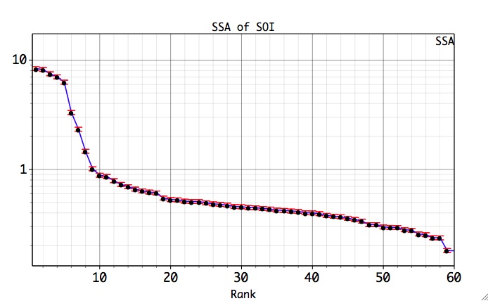
Since the window length was set to 60, SSA decomposes the time series into 60 components and thus 60 eigenvalues are plotted. The significance of the various components can be judged qualitatively by noting which components contribute significantly more variance relative to the noise background. The latter in turn assumed to include the components that lie in the flattish tail of the eigenvalue spectrum, i.e. components from about 10 to 60. The leading 10 components in a previous figure lie above a distinct break in the eigenvalue spectrum, and thus may be of physical significance.
In particular, we are interested in the leading four components which form two pairs of nearly equal eigenvalues. As discussed in the SSA theory section, pair of nearly equal eigenvalues in SSA is one that characterizing it as an oscillation. However, the eigenvalues are subject to numerical and sampling errors, and mere pairing of eigenvalues is not enough to guarantee that an oscillation has been identified. In the eigenvalue plot above, the error bars show an ad hoc range of the estimation errors. Any of the eigenvalues with significantly overlapping error bars could represent an "oscillatory pair'. Also eigenvalues with error bars that overlap significantly with the error bars of the noise part of the spectrum must also be suspected of being part of that noise.
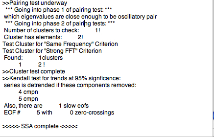
The Toolkit provides three pairing criteria to identify oscillatory pairs and trend components in clusters of eigenvalues whose ad-hoc error bars overlap; however, it is not necessary for the 'Heuristic' test to be selected on the main SSA panel. The results of these tests are can be accessed in Log tab. These tests can be activated concurrently using checkboxes in Advanced panel:
For the SOI example, the log shows that pair 1-2 of SSA components passes both `Same Frequency' and `Strong FFT' tests for being oscillation, while the 5th component is indicated as a trend (see here for more on SSA detrending):
Two fixed T-EOF bases are used using Basis popup menu in Advanced Options:
`Confidence': in percentiles, e.g. 95 will mean 95% confidence level with respect to red noise null-hypothesis.
`No. Surrogates:' Number of Monte Carlo noise realizations.
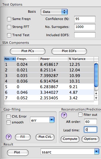
By selecting rows of the table, user can plot and inspect correspondent T-EOFs or T-PCs and perform reconstruction. In addition, SSA Prediction and Gap-filling can be performed.
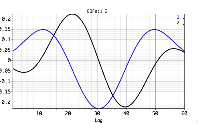
By selecting first two rows in SSA components table and clicking Plot EOFs, we can verify that the two leading EOFs are indeed in phase-quadrature, i.e. one leading the other with ~T/4 lead, where T is their common period ~40 months.
To test against a pure red-noise null-hypothesis, we choose Chi-Squared as a significance test (leaving the Included EOFs field blank). After clicking the Compute and Plot buttons, and adjusting the X-axis limits in Graph Controls window, the following plot is obtained:

Here the variance is plotted against the dominant frequencies of 'data' EOFs on x-axis, and describe projection of data and null-hypothesis (NH) surrogates onto Data EOFs basis, which are essentially SSA eigenvalues and plotted as dots. The low-frequency part of the spectrum has been zoomed in by using Graph Controls. The dominant frequencies of EOFs are calculated with a 0.001/dt resolution in the Nyquist interval from 0 to 0.5/dt. The error bars represent 95% of variance (with settings of Confidence levels such as in Advanced Options) we expect to find in the state-space direction defined by a particular EOF from the 'basis', when analyzing a segment of 'NH' noise. Using 'Included EOFS' option we can construct a composite 'NH' as described above, but it is a pure red-noise here.
For the Data Eofs basis we observe that eigenvalues corresponding to EOFS 1-2 and 3-4 appear almost superimposed on each other at frequencies equal to ~ 0.02 and 0.034 cycle/month, and lie outside the null-hypothesis error bars. Thus they are relatively unlikely ( at the 95% level set in Confidence levels of Advanced Options) to be merely due to selected null-hypothesis process, and represent two significant oscillations. The results of the Chi-squared test should always be checked using the Monte Carlo approach, which is also essential with more complex noise models.
One can also choose 'basis' EOFs to be computed from the expected covariance matrix of the 'Null-hypothesis' by selecting AR(1) from the basis popup menu in Advanced Options. Projection of data does not give SSA eigenvalues here, but the interpretation of the graph is the same. Note how the EOFs of the pure noise NH are almost regularly spaced. The NH basis avoids artificial variance-compression inherited in SSA and therefore it has a lower probability of false-positive results, i.e. identifying the noise components as significant. After doing calculations again the resulting spectrum is shown below:
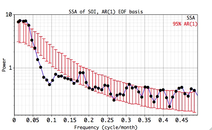
The NH basis also confirms the significance of the identified significant pairs, and we conclude that they correspond to the QB and QQ components of El Niño.
(Note: In a demo version, SSA Reconstruction/Prediction is available only for data of example projects! For custom data this feature is enabled after activation with a purchased Serial No.)
The SSA components table on the Advanced panel allows the reconstruction and prediction of the original time series from selected SSA components, as well as plotting associated T-EOFs and T-PCs by using Plot EOFs and Plot PCs buttons. The name of vector with reconstruction/prediction is specified by the user in Result field. Individual RC components are stored in matrix with name obtained by prefixing "mat_" to Result name, and can be accessed in Data I/O tool. The Result field is shared with the SSA gap-filling feature.
If results from several reconstructions have been stored in different vectors, the parameters for a particular reconstruction will be restored in GUI by simply selecting correspondent vector from Result pop-up list. For prediction user need to specify lead time in Lead field, and order of AR model to advance in time selected SSA components; cross-validation is available as well for finding optimal parameters for prediction, see SSA prediction for more details. Checking "filter out" box will filter out the selected components from the original data (prediction feature is disabled then); this can be quite useful for detrending.
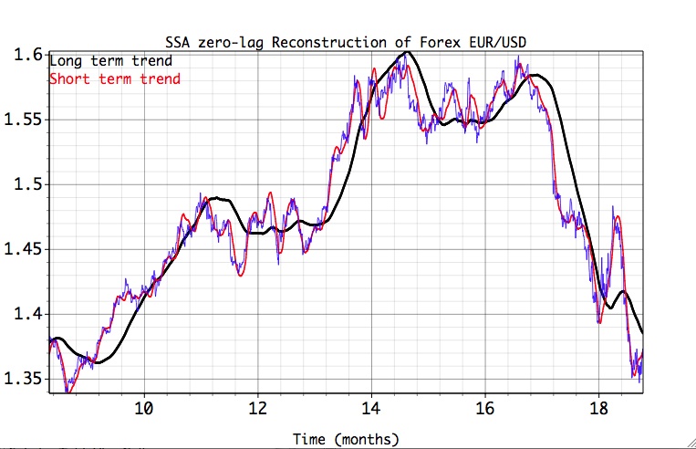
Note: By applying SSA cross-validation with Lead=0 allows to test Reconstruction feature with a fixed window size on a particular interval of the time series. The SSA is applied many times to a shortened time series, thus simulating "real-time" environment. See Finance folder in the Examples for applying this feature to the Forex USD/EUR time series.
Selecting the 1-4 table rows of identified 'significant' components , and after clicking Compute in Reconstruction/Prediction box, followed by Plot, next figure will be obtained (after adjusting its parameters in Graph Controls window):
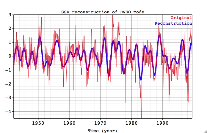
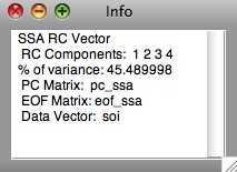
By using Info button of Vectors table in Data I/O panel, user can see the total variance captured, as well as the individual RCs used for the Result vector:
Here the reconstructed signal is plotted against original time series. If this SSA-filtered RC series is now analyzed by MEM, or MTM Coherence, the frequency spectrum of the RCs is much simpler than that of the complete time series, since most of the "noise" has been removed.We leave as an exercise for the user to repeat SSA analysis with 11 SSA Components, and try to identify pair 10-11 with the oscillatory signal. Hint: this is related to the peak in MTM Spectrum at f~0.18 cycles/month.
|
|
|
|