
 |
 |
 |
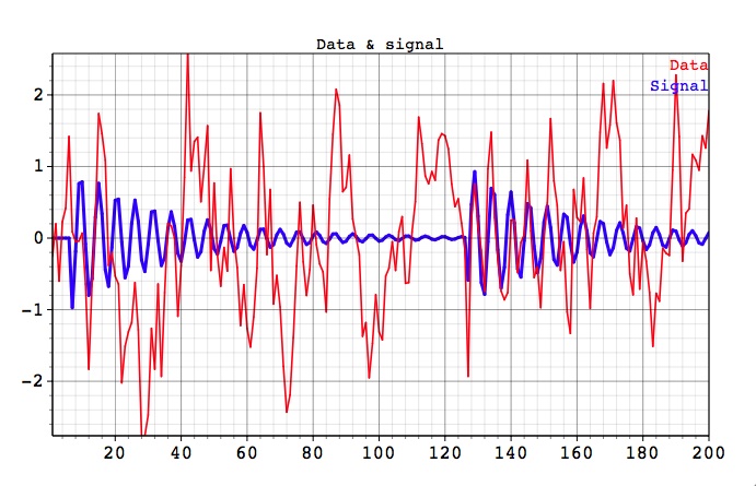
We assume that the reader is already familiar with the main SOI demo example. Here we demonstrate Toolkit capabilities to detect amplitude and phase-modulated oscillations with a very low signal to noise ratio, see Low Signal project in Examples folder of the distribution. This synthetic test series consists of randomly-generated damped oscillations bursts superimposed on large amplitude AR(1) noise. The period of the oscillations is 5.5 units, which corresponds to the frequency f=0.181. The red line in the figure below is the combined data+noise, while the blue is embedded oscillatory signal:
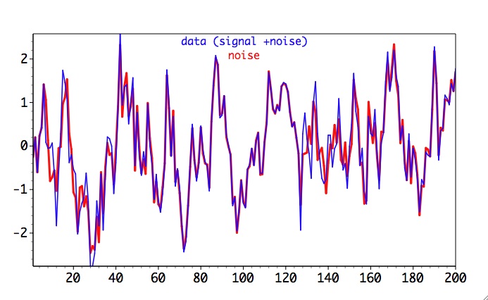
Next figure shows full data (noise + signal) against noise component only. Our task will be to identify weak oscillatory signal in this data.
Results from Blackmat-Tukey FFT applied to the full data (noise+signal) below do not show any significant peaks.
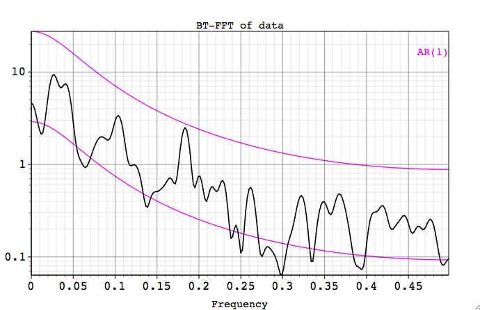
Thus we need to apply MTM and SSA methods to answer conclusively the question about any of the oscillatory peaks.
Selecting MTM from the Tools, and after clicking Default, Compute and Plot buttons, the following MTM Spectrum of the data is obtained (need to choose both Raw and Reshaped spectrum from the Plot Options):
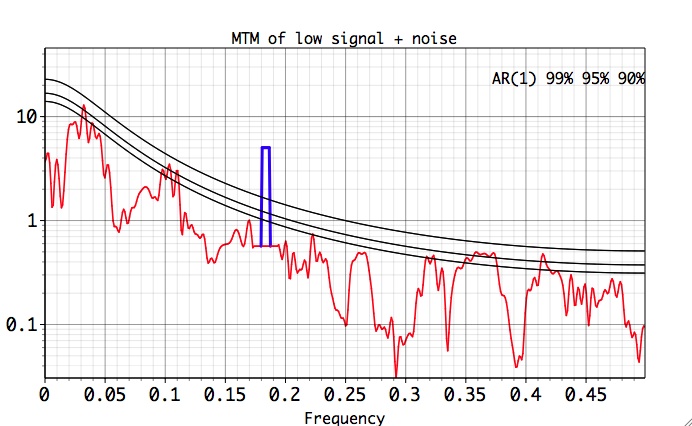
MTM Analysis
We see that MTM correctly isolates a significant oscillatory signal (blue peak) at the correct frequency ~ f=0.18. This peak passes both the MTM Harmonic test, and MTM significance test for narrowband signals against red noise. See MTM Demo for the details of the MTM analysis.
To confirm our MTM results we use the SSA analysis tool. After clicking the Default button, we change SSA window to 40, choose B&K for covariance option, select the Chi-squared quantitative significance test, 'Data' EOFs basis and test against a pure red-noise null-hypothesis by leaving Include EOFs field blank. We also check the Strong FFT and Same Frequency pairing tests in Advanced Options window, and then click the Compute and Plot buttons to obtain the following plot:
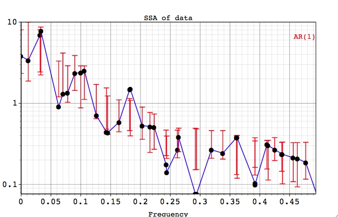
SSA: Chi-Squared Test with 'Data' EOFs
In addition, the output of pairing tests in the Log shows that EOF pair 8,9 is a candidate for oscillatory signal:
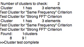
Using 'Null-Hyp Eofs' basis (AR(1) basis option ) confirms that there is significantly elevated variance in EOFS 8 and 9, which form the pair at close to the same frequency as the weak oscillatory signal in our dataset
.
As an exercise left to the user, the components with EOFS 8-9 can be reconstructed, and then passed to the MEM tool to check the frequency. Combining the results of MTM and SSA analysis, we conclude that our data contains an oscillatory signal at f=0.18.
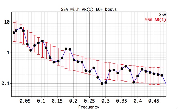
Finally, we illustrate MTM Coherence capability by computing it between full data and its noise component. The big dip at f=0.18 indicates presence of the spectral line significantly different from noise:
|
|
|
|