
 |
 |
 |
A combined SSA-MEM method can be used for time series prediction. It is started by performing SSA filtering with window M on input time-series to identify SSA "signal" components, i.e. containing oscillatory modes and/or trends. Next, we fit AR model to "signal" PCs and advance them in time to produce PCs forecasts. Finally, SSA reconstruction is performed that takes into account PCs forecasts. For small orders of AR model, forecast errors are dominated by the lack of resolution; for large orders, by the error made on the coefficients of the model. The order M is most consistent with SSA analysis, but it can be too large: the variance of the AR coefficient estimates increases with the order; M is a default value in kSpectra. Cross-validation (discussed below) can be used to identify the optimum SSA window M and AR order for prediction. Check MSSA prediction for example with multivariate data.
Here we demonstrate Toolkit capabilities to reconstruct and predict quasi-periodic oscillatory signal contaminated by noise, following prediction.tkt project in Examples/SSA Prediction folder of kSpectra distribution. The synthetic test series, 800 data points long, consists of low-frequency oscillation modulated in amplitude and contaminated by white noise.
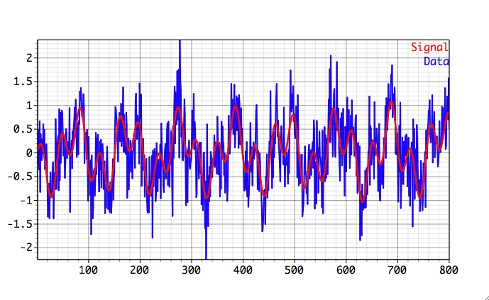
Our task will be to reconstruct and predict signal (red) from a signal+noise (blue) series. We will use Cross-Validation available in SSA Prediction Options to find optimal number of components for prediction.
We start kSpectra, and go to Data I/O in Tools. Using Finder, we double click project file prediction.tkt in SSA Prediction.
Then we go to SSA in Tools, select modul2 from Data Pop-up menu, change the Window value to M=150 (larger than longest periodicity in the time-series), and set name in Spectrum box to ssa. Then click Compute, followed by Plot, to obtain SSA spectral estimate:
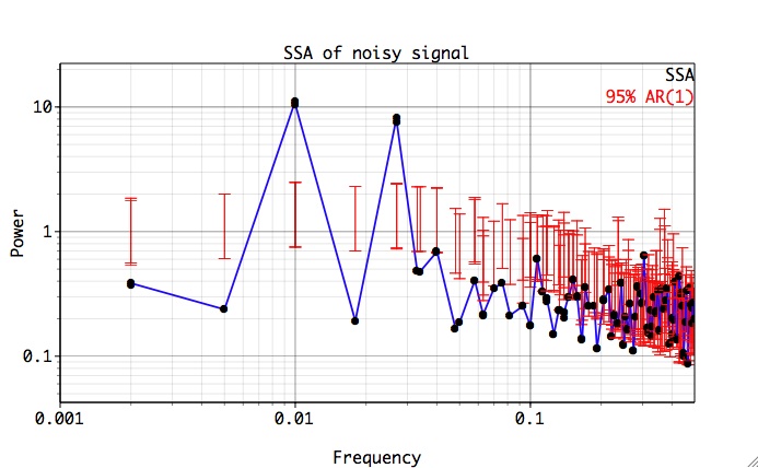
Low-frequency part of the spectrum contains a two oscillatory pairs which correspond to signal. Click Advanced options, change name in Result field to rc, and select four leading rows of SSA components table corresponding to two oscillatory pairs of the signal:
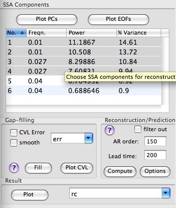
Set forecast Lead time to200, and AR order to 150 (equal to the window size).
Then we click Compute in the Reconstruction box followed by Plot to obtain Figure below:
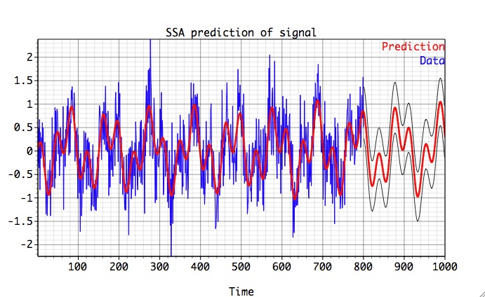
SSA prediction
If SSA cross-validation has been performed before prediction, forecast will include the confidence levels (above in black). Cross-validation is useful to access the quality of SSA forecast and optimal parameters for prediction. The basic idea is that we consider shortened time series, perform SSA forecast and compare our prediction with original record (which we know) at particular lead time.
The settings in the Reconstruction/Prediction Options for performing cross-validated forecast can be used to 1) find optimum SSA parameters for prediction and 2) provide estimates of the forecast skill.
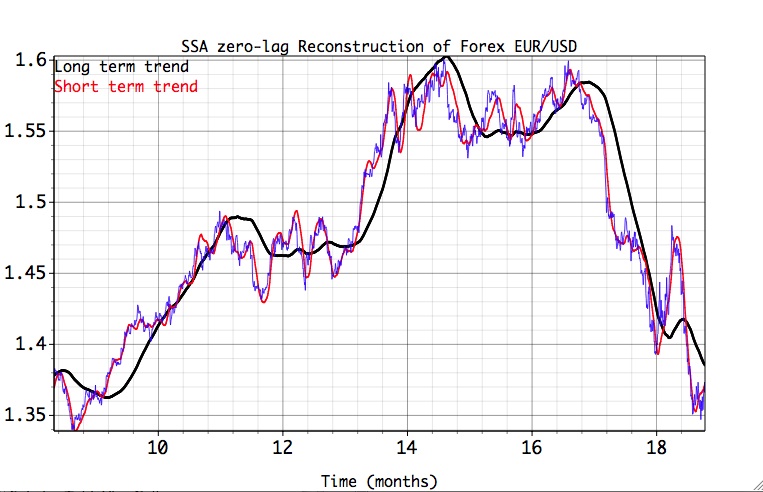
Note: By applying SSA cross-validation with Lead=0 allows to test Reconstruction feature with a fixed window size on a particular interval of the time series. The SSA Reconstruction is applied many times to a shortened time series, thus simulating analysis in "real-time" environment. See Finance folder in the Examples for applying this feature to the Forex USD/EUR time series.
We will apply cross-validation to modul2 (signal+noise) time series; please select it in the Data box of SSA tool, set on the main SSA panel number of SSA components to 6 , SSA window to 150; AR order to 150 and Lead to 200 in Advanced options, and finally in Reconstruction/Prediction Options, Start and End values of cross-validation interval to 450 (defaults to 3xSSA window size =150 in our case) and 600 (defaults to the time series length [800]-Lead [200] = 600), respectively.
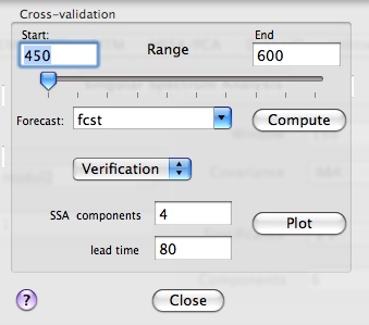
Click Compute button to calculate cross-validated forecast in this interval as a function of the lead time (up to it's maximum 200 specified in Lead) AND number of retained SSA components (up to it's maximum defined on the main SSA panel). The results of cross-validation are stored as Forecast matrix for various lead times and number of SSA components retained. In addition, forecast RMS error, anomaly correlation, as well as and Verification time series are stored as matrices with names obtained by prefixing "rms_", "cor_", and "dat_" to Forecast name, and can be accessed in Data I/O tool. Using Plot options, user can see the mean forecast skill averaged over all values of lead as a function of retained SSA components. Alternatively, user can choose to see the skill as a function of lead time for a particular number of retained SSA modes, as well as compare forecast and verification time-series (Verification option).
Results of cross-validated forecast skill for our signal+noise data are shown below:
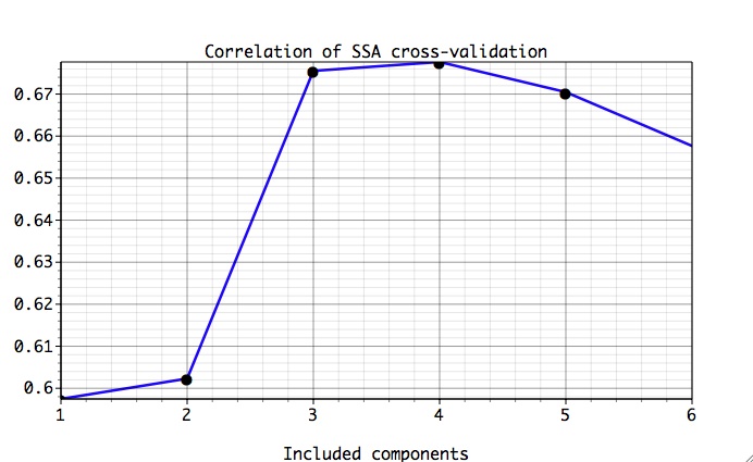
There is a maximum (minimum) of Correlation (RMS error) for four SSA components containing signal. It can be useful to vary SSA window size or/and AR order and repeat cross-validation to see if improvement in forecast skill can be obtained. To compare cross-validated time series of our SSA forecast with the data, we choose Verification option, set at the bottom of Prediction Options panel lead = 80 and number of SSA components to 4, and click Plot:
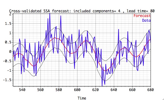
The time interval for verification plots is defined as [Start+lead,End+lead], i.e. in our case [450+80 600+80]=[530 680], and is set automatically on the verification plot by choosing appropriate transformation factors in Axes/X settings of Graph Controls. We see that our prediction generally follows the low-frequency signal, capturing quite well both it's phase and amplitude. Black confidence intervals are based on +-RMS cross-validation error at the chosen lead time. The validated time-series is bound very well within confidence levels.
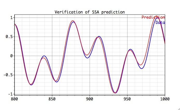
Feel free to experiment with different AR order and compare prediction results. Results of SSA prediction, naturally are dependent on amount of noise in the data, and typically improve as the amount of noise in the dataset is reduced.
The comparison of SSA predicted "signal" with its analytical enhancement is very good.
|
|
|
|