
 |
 |
 |
As an example, we apply PCA to the near-global data set of monthly sea-surface temperatures (SSTs) anomalies data set for 30° S to 60° N, on a 10° latitude x 10° longitude (International Research Institute for Climate and Society (IRI)), which translates into a dataset with 360 channels (36 longitude x 10 latitude), 648 months long. To load this dataset open project file start.tkt project in Examples/Oceanography folder.
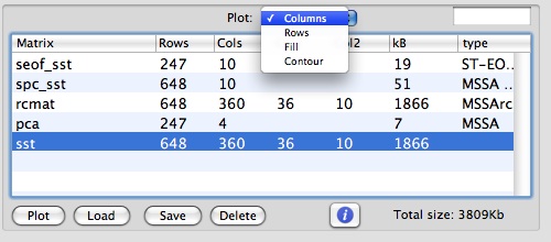
The input data is a matrix with a name "sst", which has 648 rows (time-coordinate) and 360 columns (space coordinate). The channels with NaN values in all rows indicate land mask, and there are 247 channels with actual data. User can plot column(s) or row(s) of selected matrix in Data I/O Matrices table with 1-D (Columns or Rows) or 2-D (Fill or Contour) options:
To setup a 2-D grid for display of the spatial coordinate, we can factor number of columns (cols) and set col1 and col2 values for sst matrix as 36 and 10, respectively.
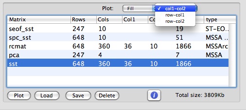
Then, all relevant MSSA (PCA) results for this matrix will be obtained and can be plotted using 2-D plot options. For Fill or Contour options, such dataset can be plotted in col1-col2, row-col1 and row-col2 coordinates. Using Fill and col1-col2 options we obtain the following plot:
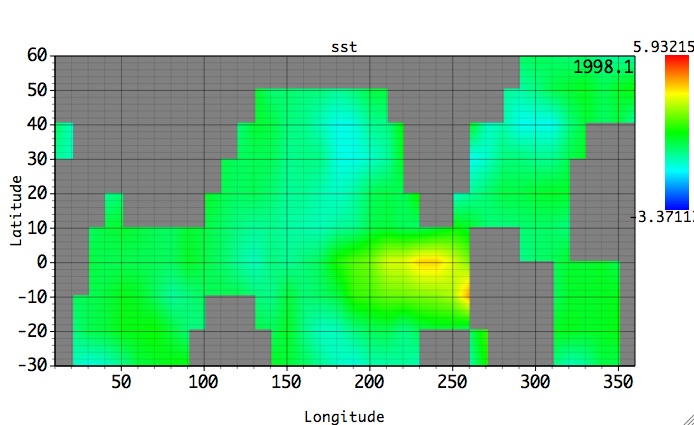
One can browse through the Z dimension of this dataset -- row (time), by going to Graph Controls/Axes/2D and using either slider, stepper or text field:
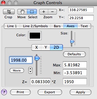
Linear transformation can be applied to the Z dimension of 2D plots in Axes/2D settings. Parameters of the transformation has to be set first. To return to the default settings, use transformation factors 1.0 and 0.0 (as in Z=1*Z + 0), or Defaults button. Above panels show how the transformation is applied to have time in calendar years, instead of months. User can also adjust the Max and Min values of the plotted field in Graph Controls/Axes/2D.
Selecting the `MSSA/PCA' tab from the Tools menu on the main panel opens the following window:
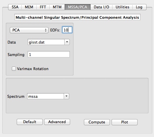
Having selected the data to be analyzed and the sampling interval, user can choose analysis type, i.e. PCA, MSSA or PCA->MSSA, which is MSSA done on data compressed by PCA.
Main option for PCA is number of spatial EOFs ( S-EOFs) to be retained for Reconstruction. Eigenspectrum of PCA is stored in matrix with a name specified in Spectrum field. In addition, S-EOFs and related principal components (PCs) are stored in matrices with names obtained by prefixing "seof_", and "spc_" to a Spectrum name, and can be accessed in Data I/O tool. If results from several analyses have been stored in different matrices, the parameters used in a particular computation will be restored in GUI by simply selecting correspondent matrix from a Spectrum pop-up list.
A VARIMAX rotation is a change of coordinates used in PCA that maximizes the sum of the variances of the S-EOFs and for this example we leave this box unchecked.
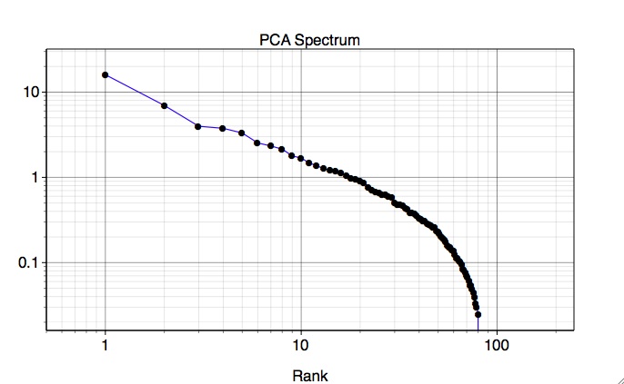
The leading spatial EOF describes 22.2% of the variance, as we can see in PCA components table of Advanced options:
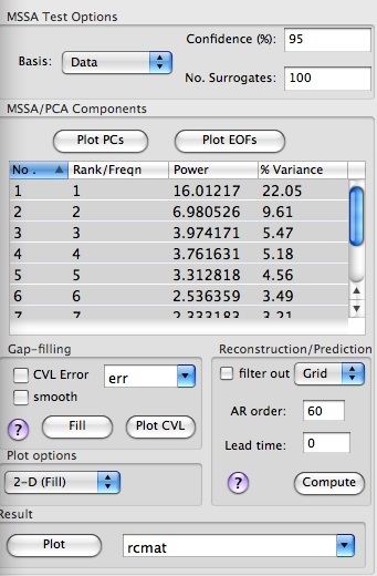
We can plot EOFs and PCs from PCA analysis by selecting multiple rows from MSSA/PCA components table, setting a Plot option, i.e. 1-D, or 2-D mode (Fill or Contour), and hitting a Plot PCs or Plot EOFs button. Note, that only 1-D plot option is available for plotting PCs.
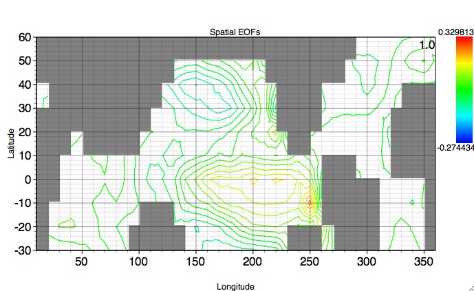
Figure above shows leading EOF (1st row in PCA table) plotted as 2-D Contour. Contour thickness can be adjusted by the Line1, number of contours by Line2, while max and min can be set in Axes/2-D of of Graph Controls, respectively. For 2-D factored (i.e x*y or col1*col2) datasets like in this example, multiple S-EOFs are plotted as one array in a single plot; user can select which EOF to show by using either slider, stepper or text field of Z dimension in Graph Controls/Axes/2D.
Associated principal component with the 1st EOF is shown below:
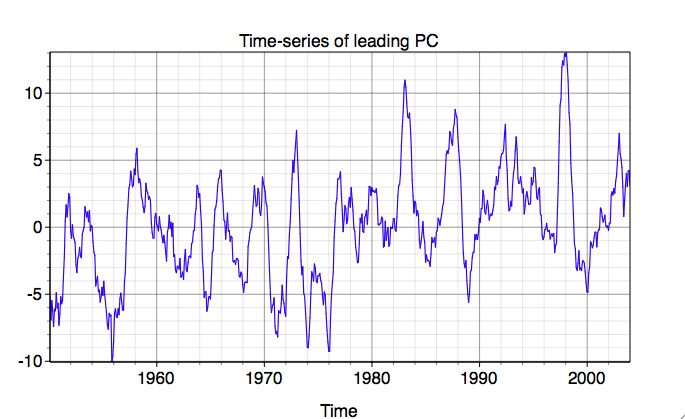
We can reconstruct contributions from selected principal components in PCA table of Advanced options panel. The name of the matrix with reconstruction is set by the user in Result box at the bottom of Advanced options. By clicking Plot there, user can compare reconstruction vs. original data in the specified column (spatial channel) or row (time channel) by using 1-D Plot Option. If 2-D Plot Option has been chosen (Contour or Fill), only reconstruction will be plotted in 2-D time-space coordinates. If the spatial dimension of input dataset has been 2-D factored (i.e x*y or col1*col2) using col1 and col2 in Matrices table of Data I/O, the space-time reconstruction will be displayed in x-y as well, with a time coordinate becoming Z dimension.
The figure below shows plot of reconstruction using 2-D Fill plot option:
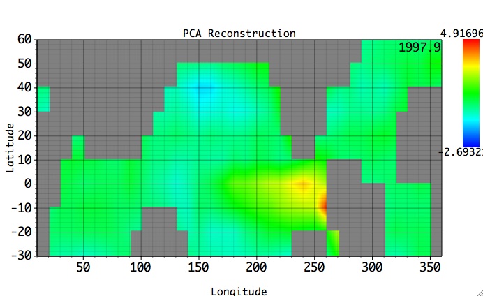
We can browse through the Z dimension of this dataset -- time, and apply linear transformation to it, by using either slider, stepper or text field in Graph Controls/Axes/2D.
Checking "filter out" box in Options of Reconstruction will filter out the selected components from the original data; this can be quite useful for detrending. If results from several reconstructions have been stored in different matrices, the parameters for a particular reconstruction will be restored in GUI by simply selecting correspondent matrix from a Result pop-up list.
|
|
|
|