 |
 |
The MultiTaper method (MTM) of spectral analysis provides a novel means for spectral estimation (Thomson, 1982; Percival and Walden, 1993) and signal reconstruction (e.g., Park, 1992) of a time series which is believed to exhibit a spectrum containing both continuous and singular components. This method has been widely applied to problems in geophysical signal analysis, including analyses of atmospheric and oceanic data, paleoclimate data, geochemical tracer data, and seismological data.
MTM, like the method of Blackman and Tukey, offers the appeal of being nonparametric, in that it does not prescribe an a priori (e.g., autoregressive) model for the process generating the time series under analysis. MTM attempts to reduce the variance of spectral estimates by using a small set of tapers rather than the unique data taper or spectral window used by Blackman-Tukey methods. A set of independent estimates of the power spectrum is computed, by pre-multiplying the data by orthogonal tapers which are constructed to minimize the spectral leakage due to the finite length of the data set. The optimal tapers or ``eigentapers'' belong to a family of functions known as discrete prolate spheroidal sequences (DPSS) which are defined as the eigenvectors of a suitable Rayleigh-Ritz minimization problem. Averaging over this (small) ensemble of spectra yields a better and more stable estimate -- i.e., one with lower variance -- than do single-taper methods. The tapers are the discrete set of eigenfunctions which solve the variational problem of minimizing leakage outside of a frequency band of half bandwidth pfn where fn=1/Ndt is the Rayleigh frequency, and p is an integer.
In practice, only the first 2p - 1 tapers provide usefully small spectral-leakage, and thus the number of tapers used K should be less than 2p-1 in any application of MTM. The choice of the bandwidth 2pfn and number of tapers K thus represents the classical tradeoff between spectral resolution and the stability or ``variance'' properties of the spectral estimate. The trivial case K=1 and p=1 is, again, the single-tapered DFT of Blackman and Tukey.
For typical length instrumental climate records, the choice K=3, p=2 offers a good compromise between the required frequency resolution for resolving distinct climate signals (e.g., ENSO and decadal-scale variability) and the benefit of multiple spectral degrees of freedom. Longer datasets can admit the use of a greater number K of tapers while maintaining a desired frequency resolution, and the optimal choice of K and p is in general most decidedly application specific.
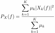
MTM can provide estimates of both the singular components (i.e, the ``lines'') and the continuous component (ie, the background) of the spectrum. Once the tapers wk(t) are computed for a chosen frequency bandwidth, the total power spectrum PX can be estimated by averaging the individual spectra given by each tapered version of the time series x(t); the kth eigenspectrum Xk is the DFT of x(t)wk(t) . The high-resolution multitaper spectrum is a simple weighted sum of the K eigenspectra,

and the weights &muk are based on the eigenvalues from the DPSS solution. The ``line'' components in high-resolution spectrum will be detected as peaks or bumps of width 2pfn. For a white noise or ``locally white noise'' process the high-resolution spectrum is chi-squared distributed with 2K degrees of freedom.
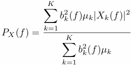
By adjusting the relative weights on the contributions from each of the K eigenspectra, a more leakage-resistant spectral estimate termed the adaptively weighted multitaper spectrum is obtained,

where bk(f) is a weighting function that further guards against broadband leakage for a non-white (``colored'') but locally-white process. The adaptive spectrum estimate has an effective degrees of freedom that generally departs only slightly from the nominal value 2K of the high-resolution multitaper spectrum.
The purpose of harmonic analysis is to determine the line components-ie the spikes in the spectrum corresponding to a periodic or quasi-periodic signal-in terms of their frequency, amplitude, and phase. The Fourier transform of a clean periodic signal of infinite length yields a Dirac function at the frequency of the signal, viz., a line (or peak of zero width) with infinite magnitude. A spectral estimate based on the methods discussed in earlier sections, gives indirect information on the amplitude of the signal at a given frequency, through the area under the peak centered at that frequency and whose width is, roughly speaking, inversely proportional to the length N of the time series; this area is nearly constant, since the height of the peak is also proportional to N. Harmonic analysis attempts, instead, to determine directly the (finite) amplitude of a (pure) line in the spectrum of a time series of finite length. We explain next how this is done within MTM.
Assume the time series x(t) is the sum of a sinusoid of frequency f0 and amplitude B, plus a ``noise'' &eta(t) which is the sum of other sinusoids and white noise. One can then write
![]()
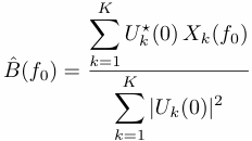
If (wk(t), k=0, ......K-1) are the first K eigentapers and Uk(f) is the DFT of wk(t), a least-square fit in the frequency domain yields an estimate of the amplitude B:

where the asterisk denotes complex conjugation. A statistical confidence interval can be given for the least-squares fit by a Fisher-Snedecor test, or F-test. This test is roughly based on the ratio of the variance captured by the filtered portion of the time series x(t), using K eigentapers, to the residual variance. By expanding the variance of the model one finds that it is the sum of two terms,
and

that are respectively the ``explained'' and ``unexplained'' contributions to the variance.
The random variable

would obey a Fisher-Snedecor law with 2 and 2K-2 degrees of freedom if the time series x(t) were a pure white-noise realization. One can interpret its numerical value for given data by assuming that B=0 -- i.e., that x(t) is white- and trying to reject the white noise null hypothesis. In practice, the spectrum need only be ``locally white'' in the sense that the K eigenspectra which describe the local characteristics of the spectrum should be distributed as they would be for white noise.
This harmonic-analysis application of MTM is able to detect low-amplitude harmonic oscillations in a relatively short time series with a high degree of statistical significance or to reject a large amplitude if it failed the F-test, because the F-value F(f) does not depend -- to first order -- on the magnitude of B(f). This feature is an important advantage of MTM over standard methods where error bars are essentially proportional to the amplitude of a peak. However, the implicit assumption in the harmonic-analysis appproach is that the time series is produced by a process that consists of a superposition of separate, purely periodic fixed-amplitude components. If not, a continuous spectrum (in the case of a colored noise or a chaotic system) will be broken down into spurious lines with arbitrary frequencies and possibly high F-values. In essence, the above procedure assumes that ``signals'' are represented by lines in the spectrum corresponding to phase-coherent harmonic signals, while the ``noise'' is represented by the continuous component of the spectrum. In geophysical applications, signals are frequently associated with narrowband, but not strictly harmonic variability and truly harmonic signals are rarely detected. In such cases, the simple noise null hypothesis and signal assumptions implicit in the traditional MTM approach described above loses much of its utility.
The more subtle nature of geophysical signals and noise has led to a more recent generalization of the conventional MTM approach which combines the harmonic signal detection procedure described above, with a criterion for detecting significant narrowband, ``quasi-oscillatory'' signals which may exhibit phase and amplitude modulation, and intermittent oscillatory behavior, but are nonetheless significant relative to some suitably defined null hypothesis. We favour this approach, whichs provides for the detection and significance estimation of both harmonic and anharmonic, narrowband signals in the MTM spectra of time series, making use of a ``robust'' estimate of the background noise.
Information from the harmonic peak test of the traditional MTM procedure is retained, but peaks, whether indicated as harmonic or anharmonic, are tested for significance relative to the null hypothesis of a globally red (or, trivially, white) noise background estimated empirically from the data. This is particularly important in climate studies, where the intrinsic inertia of the system leads to greater power (and greater liklihood of prominent peaks in the spectrum) at lower frequencies, even in the absence of any signals. To accomodate the red noise background assumption requisite in geophysical applications, an AR(1) noise process is assumed, although more complex noise models can be motiviated.
The power spectrum of the AR(1) process is given by:
 ,
,
where P0 is the average value of the power spectrum, related to the variance &sigma by,
![]()
while r is the lag-one autocorrelation, and fN=0.5/dt , the Nyquist frequency, is the highest frequency that can be resolved for sampling rate dt . The characteristic noise decay time scale can be estimated

For periodicities much larger than &tau, the spectrum behavies like a white spectrum.
The approach of Mann and Lees (1996) performs a ``robust'' estimate of the red noise background by minimizing (as a function of r) the misfit between an analytical AR(1) red noise spectrum and the adaptively weighted multitaper spectrum convoluted with a median smoother. The median smoothing operation in the fit insures that the estimated noise background is insensitive to outliers (most obviously, peaks associated with signals) that, properly, should not influence the estimation of the global noise background. This guards against the typical problem of inflated estimates of noise variance and noise autocorrelation that arise in a conventional Box-Jenkins approach due to the contamination of noise parameters by non-noise contributions (e.g., a significant trend or oscillatory component of the series). Mann and Lees (1996) motivate the choice of a median smoothing width of &Delta f =min(fN/4, 2pfn) as a compromise between describing the full variation of the background spectrum over the Nyquist interval, and insensitivity to narrow spectral features.
Significance levels for harmonic or narrowband spectral features relative to the estimated noise background can be determined from the appropriate quantiles of the chi-squared distribution, approximating the spectrum as being distributed with 2K degrees of freedom. A reshaped spectrum is determined in which the contributions from harmonic signals are removed, depending on a significance threshold for the F variance-ratio test described above. In this way, noise background, harmonic, and anharmonic narrowband signals are each independently isolated. The harmonic peak detection procedure provides information as to whether the signals are best approximated as harmonic (phase-coherent sinusoidal oscillations) or narrowband (amplitude and phase modulated, perhaps intermittant oscillations). In either case, they must be significant relative to a specified (e.g., red) noise hypothesis to be isolated as significant.
Once significant peaks have been isolated in the spectrum, relative to the specified null hypothesis, the associated signals can be reconstructed in the time domain using the information from the multitaper decomposition. The signals or ``reconstructed components'' are analagous to those of SSA described in previous sections, except that information from a frequency domain eigendecomposition, rather than a correlation-domain eigendecomposition, is used to reconstruct the detected signal. As in the correlation-domain case, a priori assumptions regarding the domain boundaries must be invoked.
The reconstructed signal corresponding to a peak centered at frequency f0 can be obtained as
![]() ,
,
where the envelope function A(t) is determined from a time-domain inversion of the spectral domain information contained in the K complex eigenspectra. The envelope A(t) has K complex degrees of freedom, and allows for phase and amplitude variations in the time reconstruction of the signal centered at frequency f0. The discrete time sequence describing the complex envelope An is determined from a discrete inverse problem using the complex amplitudes of each of the the K eigenspectra and appropriate boundary conditions. The three lowest order boundary contsraints in this inversion involve minimization of the envelope An itself near the boundaries, numerical mimimization of the slope of the envelope near the boundaries, or optimization of the smoothness of the envelope (ie, numerical minimization of the 2nd derivative near the boundaries). Any one of these choices might be favoured if a priori information regarding the characteristics of the signal is available. The amplitude of the seasonal cycle in surface temperature, for example, is nearly constant in time, and a minimum slope constraint is most appropriate for its reconstruction. Generally, however, a nearly optimal reconstruction can always be obtained through seeking the weighted linear combination of these 3 contraints that minimizes the mean-square misfit of the reconstructed signal with respect to the raw data series. We favour this method of time-domain inversion.
Magnitude-squared coherence CXY is a function of frequency with values between 0 and 1, and is a fraction of a common variance between two time series x and y through a linear relation. It is defined by using the individual power spectra estimates (PX and PY ) of x and y and the cross-power spectrum PXY:

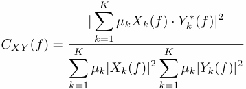
In practice,CXY has to be computed by using some kind of time-frequency ensemble averaging. Multitaper method with K tapers provides a practical way to compute CXY by using the individual DFT estimates Xk and Yk of data x and y tapered with k-th taper:

The confidence limits of estimated coherence at a given level &alpha (95% is &alpha=0.05) can be calculated as:
![]()
Cross-power spectrum PXY can be obtained with Blackman-Tukey method. Multi-channel SSA is an advanced, data-adaptive method to analyze oscillatory spatio-temporal modes in multivariate time series. In addition to identifying oscillatory peaks in the cross-spectrum, MSSA allows reconstruction of the multivariate oscillatory modes.
1. Mann, M.E. and Lees, J.M., 1996: Robust estimation of background noise and signal detection in climatic time series, Clim. Change., 33, 409-445.
2. Percival, D.B., and Walden, A.T., 1993: Spectral analysis for physical applications--Multitaper and conventional univariate techniques. Cambridge University, 580 pp.
3. Park, J., 1992: Envelope estimation for quasi-periodic geophysical signals in noise: A multitaper approach, in Statistics in the Environmental and Earth Sciences, edited by A.T. Walden and P. Guttorp, 189-219, Edward Arnold, London.
4. Thomson, D.J., 1982: Spectrum estimation and harmonic analysis, Proc. IEEE, 70, 1055-1096.