 |
 |
 |
Double-click `kSpectra', and the Start-up window will appear:
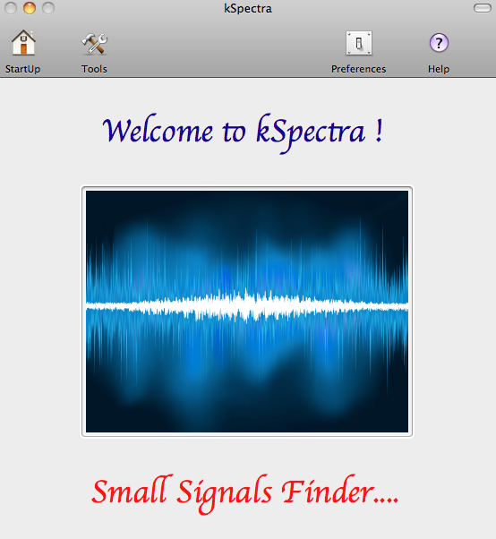
By using the toolbar you can access the following functions of the toolkit:
FFT: Blackman-Tukey Correlogram and Cross-Spectra
MEM: Maximum-Entropy spectrum estimation
MTM: Multi-Taper Method spectrum estimation and Coherence
SSA: Singular Spectrum Analysis
MSSA/PCA: Multi-channel Singular Spectrum and Principal Component Analysis
Data I/O: loads, saves, and plots of vector and matrix data
Utilities: useful utilities for multi-vector plots, comparing spectra, and managing data
Log : shows the internal log file containing the detailed output from all tools
We will work through examples using each tool on a univariate time series of monthly values of the Southern Oscillation Index (SOI), a climatic index that characterizes El Niño (Bjerknes, 1969), see Climate example in the distribution.
The 690 month series was obtained from monthly mean sea-level pressures at Tahiti and Darwin, Australia, by removing their seasonal cycles, dividing the resulting anomalies by the corresponding standard deviations, and then taking the Tahiti-minus-Darwin difference. The SOI series considered here is for the time interval from January 1942 through June 1999, during which no observations are missing. The complete project of analyzing SOI time series can be found in Examples/Climate folder of kSpectra distribution. Next figure shows the 'Data I/O' panel for data in soi.tkt after double-clicking on it in a Finder:
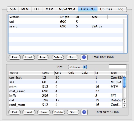
kSpectra Toolkit allows you to handle many time series at once; these might typically be a raw input time series, spectral analysis results, and filtered series derived using the Toolkit. These time series are stored as Vectors or Matrices, which are named data objects. The Matrices and Vector tables provide information about their names, dimensions, i.e. the number of elements in a vector (length) and number of rows and columns for a matrix (rows and cols). The total size of the data object in kB as listed, as well as it's type. The empty type is reserved for imported data, while the type is usually set for the results of kSpectra analysis, such as "MEM", "FFT", "EOFs of SSA", or "SSArcs".
For Matrices representing 2-D spatial multivariate time series (X-Y), it is possible to setup a 2-D grid for by factoring number of columns (cols) and set col1 and col2 values as col=col1*col2, where col represents the total number of spatial points, and col1 and col2 refer to 2-D dimensions X and Y, respectively. This feature is extremely useful for visualization of PCA/MSSA results, and users can setup a 2-D grid in the correspondent columns of Matrices table .
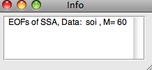
which tells that this matrix contains Empirical Orthogonal Functions (EOFs) of SSA applied to data vector soi with a window M=60.
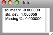
For Matrix with M columns and named "name", the basic statistics is computed for its columns and stored in new matrices with one row and M columns, named as "name_mean", "name_stddev", "name_miss", and with a type "Mean", "StdDev" and "Miss", respectively.
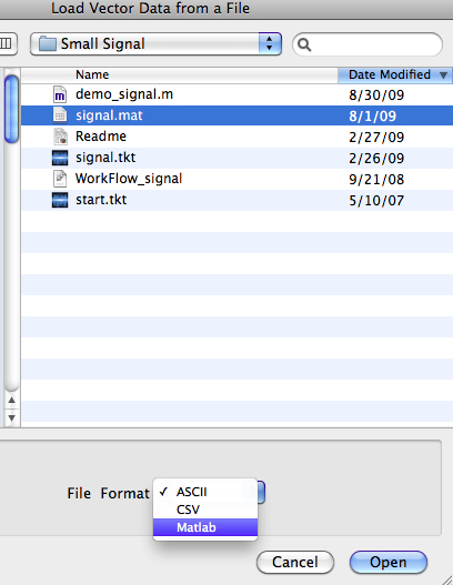
Data I/O is supported for ASCII, CSV (comma-separated-values) and Matlab formatted files. Input files should contain only numerical data. The time series can be imported for analysis using the `Load' button in Vectors (Matrices) table views, or just simply by performing Drag-and-Drop operation of the file from Finder to the relevant table view.
The time series must be equally spaced in time. The value of sampling interval is assumed to be 1 (unity) by default, or the sampling interval can be set by using the "Sampling" fields for each spectral tool individually. The resulting spectral estimates are then plotted accordingly. If, for example, the input data are sampled every 2 months, the Nyquist interval on the frequency axis will be labeled from 0 to 0.25 cycles/month. File data with NaN values (case insensitive) are treated as missing. To analyze such data Univariate Gap-Filling and Multivariate Gap-filling methods are provided.
If the data is read from ASCII or CSV files, new Vector or Matrix data object will have a file's name. The names of data objects can not be changed once created, but new data objects can be changed and copied with Manage Data utility.
Data objects can be also saved using the `Save' button or by dragging out selected rows in Vectors (Matrices) table views to Finder (available only in a licensed copy of kSpectra Toolkit). The user then can the choose the desired ouput format - ASCII, CSV or Matlab In the latter case the single file will be created for all the selected data objects. To save all data in a single Matlab file use Save MAT-file option in File Menu (see below).
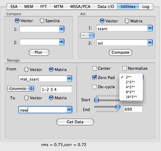
Utilities
Compare
Compare utility compares on the same plot two selected vectors or spectral estimates.
Manage
Manage utility allows to copy specified Columns (Rows) of Matrices, or Vector, from a source data object selected in From section, to a new target data object, whose type and name is set in To section.
If Columns (Rows) field is left empty, then by default all Columns (Rows) of the source Matrix will be copied to a target Matrix. Contiguous Columns (Rows) of a Matrix source can be specified individually, i.e. 1 2 3 4, or in concise form as 1-4. The Start and End sliders control the range of copied data: if source is a Vector, then it is the range of its indices. If source is a Matrix and its Columns are copied, sliders will control number of Rows in a target, and visa versa.
In addition, the following optional operations can be performed on the target (if it is a Matrix, these options will act on its columns):
Act
Act utility will perform various operations between two selected data objects.
If "+" or "-" action is chosen, it computes sum or difference of the two objects, respectively. The result is stored in a new data object with a name derived from the names of its sources, i.e. "name1+name2" or "name1-name2". The selected data objects should have the same sizes, i.e. length for Vectors, and number of rows and columns for matrices. In addition, root-mean-squared (rms) of the result and correlation (corr) of the source objects, is computed. For two selected Vectors, rms and corr are two scalars which are displayed at the bottom of kSpectra window (see above) and also recorded to Log.
For two selected Matrices, rms and corr are computed column-wise; the results are stored in matrices having one row, and named as "name1+name2_rms" (or "name1-name2_rms") and "name1+name2_corr" (or "name1-name2_corr"), respectively. Column averaged rms and corr are displayed at the bottom of kSpectra window as well.
The [ ] action will merge two data objects (Vectors or Matrices) by columns, side by side. The selected data objects should have the same dimensions, i.e. length for Vectors, and number of rows for matrices. The result is stored in a new matrix with a name derived from the names of its sources, i.e. "name1[ ]name2", and will have two columns if Vectors are merged, and combined number of columns of two sources, if Matrices are merged,
For Matrices two additional actions are provided to use the output of the Stat function in Data I/O (see above). The ".*" action can perform renormalization of Matrix 1 by multiplying its columns by the values of a single row of Matrix 2, which is automatically filtered to be of type "StdDev". The ".+" action will filter in Matrix 2 only matrices of type "Mean", and adds values of its single row to columns of Matrix 1. The number of columns should be equal in both matrices.
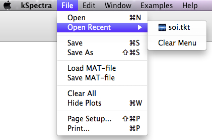
Single projects files containing all data and plots, can be opened and saved with Open, Open Recent, Save and Save As menu features (saving is available only in a licensed copy of kSpectra Toolkit). By default the project file is given the .tkt extension. Clear All option removes all the data from the application's memory and closes all the windows with plots. Hide Plots option closes all the plots.
Load Mat-file and Save Mat-file options support data I/O to Matlab (saving is available only in a licensed copy). Matlab scripts for plotting kSpectra results are provided with Demo version.
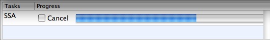
At the bottom of the main window there is a drawer Task Manager which is usually hidden. It opens only when the analysis has been started with any of the tools, or I/O operations are performed, and an entry appears in the Task Manager with a progress bar. The user can stop any task by checking a Cancel flag next to a progress bar:
When there are no active computation tasks running, the Task Manager drawer closes.
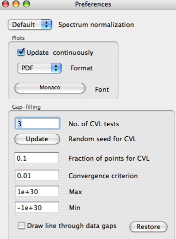
Preferences
There are three options for spectrum normalization throughout the Toolkit that can be selected in Preferences panel in kSpectra menu. The default option is for the power spectrum to be normalized by the length of the time series - (InputUnit)2. Next is power spectral density (PSD) which is the power spectrum divided by the frequency range - (InputUnit)2/Hz, and finally the square-root of PSD.
User can choose EPS or PDF file format for saving plots, and the default font for labels and legends. If "Update plot continuously" is checked, any change in Graph Controls settings is applied immediately to the ActivePlot (see below). If it is unchecked, user can adjust several settings and then apply all the changes to ActivePlot at once with Apply button.
Also, number of cross-validation tests for gap-filling can be set here (see MSSA and SSA gap-filling sections), as well as option to connect points (linear interpolation) through gaps when plotting datasets with missing data. Restore option return default Preference values.
|
|
|
|