
 |
 |
 |
To make a plot of the vector time-series data, we can use the 'Data I/O' panel in Tools, by selecting vector soi from the table and pressing on the 'Plot' button:
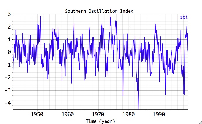
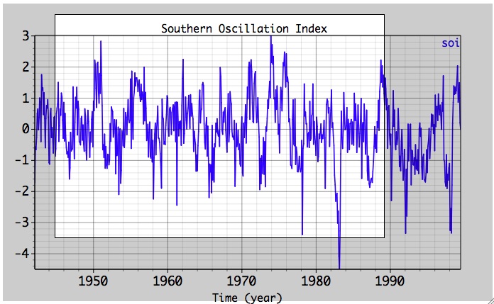
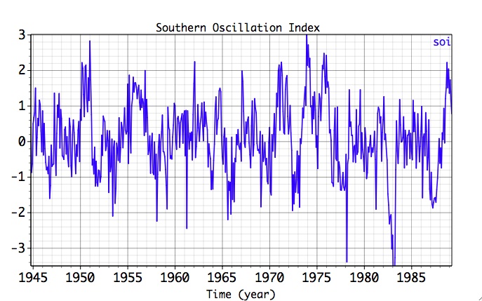
The SOI time series is noisy, with no obvious oscillatory components. Our goal is to identify the low-frequency quasi-quadrennial (QQ) and quasi-biennial (QB) components of El Niño (Rasmusson et al., 1990).
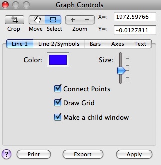
Double-clicking on any graph window makes it an Active plot and brings forward adjacent Graph Controls window, where the properties of the Active plot can be changed by choosing tabs Line 1, Line2/Symbols, Bars, Axes and Text. Not all the
If "Update plot continously" is checked in Preferences panel, any change in Graph Controls settings is applied immediately to the ActivePlot. If it is unchecked, user can adjust several settings and then apply all the changes to ActivePlot at once with Apply button. By default, the Graph Controls window is a "child window" of an Active Plot; user controls this option by using the switch button (see on the left panel below):
 |
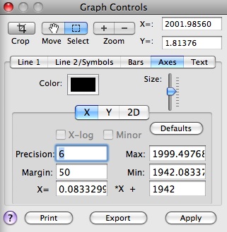 |
Placement and labelling of major and minor axis ticks marks is performed automatically for linear axes. Major ticks are labeled according to the specified Precision, while Margin number in pixels controls Left and Right (Axes/X) and Top and Bottom (Axes/Y) plot margins. For plots with spectral estimates (SSA, MEM, BK-FFT and MSSA) users can use X-log or/and Y-log coordinate transformations in respective Axes tab; when Log transformation is applied user can choose also to plot labels at minor ticks.
Linear transformation can be applied to the abscissa of data plots in Axes/X settings (and for ordinate of 2-D data plots in Axes/Y settings). Parameters of the transformation has to be set first; new Xmin and Xmax values will be updated automatically. User can then adjust Xmin and Xmax as desired. To return to the default abscissa settings, use transformation factors 1.0 and 0.0 (as in X=1 *X + 0), or Defaults button. Above panels show how the transformation is applied to have abscissa in calendar years in the plot of SOI time series shown before, instead of default index (which for SOI is in months).
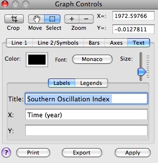
Settings for Labels, Title and Legends can be specified in the Text tab:
 |
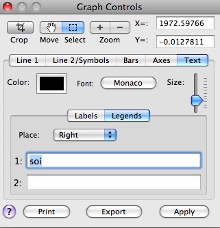 |
By clicking on a Font button in Text tab, a font panel is brought forward where current font selection of Active Plot can be changed; the default font for new plots can be set in Preferences panel. Users can see coordinates of a point clicked by a mouse at the top of GraphControls, export current ActivePlot in EPS or PDF format (set in Preferences panel), and Print it. Orientation settings for printing are specified in Page setup item of a File menu.
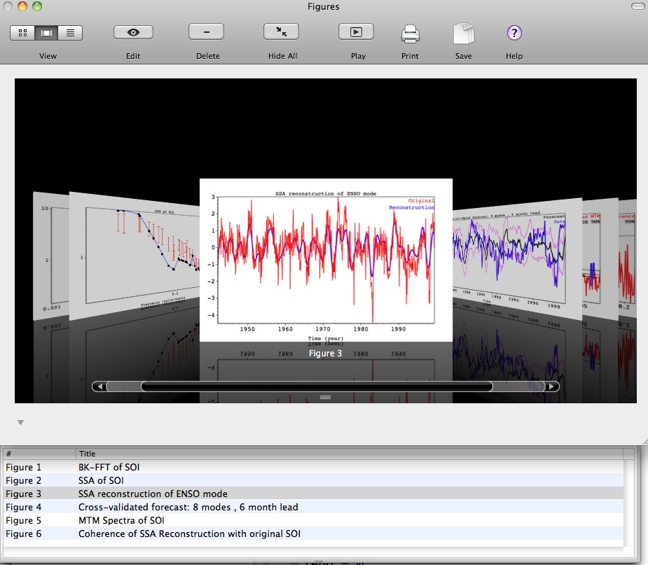
Version built exclusively for Mac OS 10.5+, provides a convenient way to store, access and manage multiple Plots using a separate window called Gallery. The plots can be accessed there by using thumbnails in three different ways: Browser View, Cover Flow View (similar to iTunes), or by table List View. The View type can be changed in the toolbar of the Gallery. The table List View can be also accessed in Cover Flow and Browser Views by the triangle disclosure button.
Cover Flow View:
Browser View:
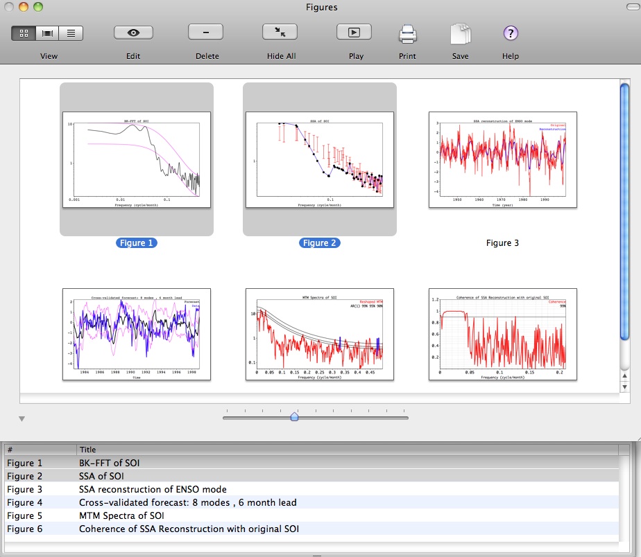
The slider on Browser View controls size of Plots thumbnails which can be rearranged by dragging.
List View:
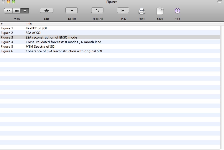
User can navigate and do different selections in any of the Views by using Arrow-Up, Arrow-Down, Arrow-Let and Arrow-right keys. One or more individual plots can be retrieved from a Gallery and made Active Plot(s) by selecting it in any of the Views, and then either clicking Edit at the toolbar of the Gallery, or by pressing Space bar of the keyboard, or by double clicking in Browser or List Views. To hide the Active Plot(s) again in the Gallery simply click yellow button at the left corner of Active Plot's window, or use Hide All in the toolbar or Option+W keyboard combination. Saved project files retain information about Active Plots that were open outside the Gallery at the tme of saving, and will display them accordingly when the files are loaded.
To erase selected Plot(s) completely either click Delete button at the Gallery's toolbar, click red button at the left corner of Active Plot's window, or use Delete key of keyboard.
To view slideshow of selected Plots in full screen mode click Play on the Gallery's toolbar.
To print selected Plots click Print buton in the Gallery's toolbar.
To save selected Plots to the disk in EPS or PDF format click Save buton in the Gallery's toolbar.
When mouse cursor is moved over the Active plot, its current coordinates are tracked and displayed in X and Y fields at the top of GraphControls. The Zoom tool allows to gradually zoom in/out from the center of the Active Plot. Dragging a mouse over the Active Plot is controlled by Select and Move options of Drag button. When Select option is chosen in Graph Controls, a portion of the plot can be selected by dragging mouse over the ActivePlot, and then cropped by using Crop button in GraphControls:
When Move button is pressed in Graph Controls, dragging a mouse forces continuous change of the ActivePlot max and min limits; this effect can be also achieved by using Arrow keyboard strokes (Up, Down, Left and Right). To avoid unwanted Move simplyclick Select option.
User can plot column(s) or row(s) of selected matrix in Data I/O Matrices table with Columns or Rows options, or plot them with 2-D Fill or Contour options. Following figure is for the example from multivariate gap-filling.
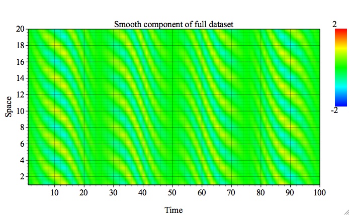
Contour thickness can be adjusted by Line1, and number of contours by Line2 settings of Graph Controls, respectively. The maximum and minimum values of plotted field is adjusted by Graph Controls/Axes/2D settings:
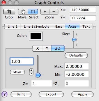
See other multivariate examples in PCA and MSSA for 2-D plotting when Columns are considered to be a spatial coordinate corresponding to a rectangular grid; in this case plot can be browsed by rows, can be animated and saved to a QuickTime movie.
|
|
|
|