
 |
 |
 |
|
|
|
|
Once a data vector has been read in using Data I/O, we choose `FFT' from the Analysis.
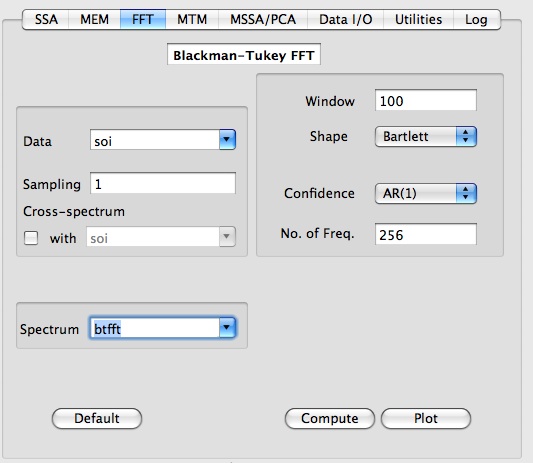
Here the user needs to specify the vector name of the data to be analyzed, the value of the sampling interval dt, the window type and size, as well as the number of sample frequencies to be plotted. Default values can be specified by pressing Default button. If the sampling interval is not specified, it is set to default value equal to 1. Results of BT-FFT analysis are stored in matrix with a name specified in Spectrum field. If results from several BT-FFT runs have been stored in different matrices, the parameters used in a particular BT-FFT analysis will be restored in GUI by simply selecting correspondent matrix from a Spectrum pop-up list.
The Window type pull-down menu allows one to choose the shape of the windowing function to be applied in estimating the correlogram. The window shapes available are:
As Press et al. (1989) have noted, the choice of window functions is usually not as important as the choice of Window Size. The Default button allows a default choice of window size and the number of sample frequencies. The latter is forced by the Toolkit to be equal to a power of 2, and evenly-spaced between 0 and the Nyquist frequency 0.5/dt, where dt is the sampling interval of the data entered by the user in the Sampling field. Thus, the units of the abscissa on all plots are cycles per sampling interval, over the range 0 to 0.5/dt.
The smaller the window size, the more independent samples are obtained for estimation purposes and therefore the smaller will be the variance of the spectral estimate. However, the smaller the window size, the lower the spectral resolution of the estimate will be. Note that the spectral resolution is independent of the number of sample frequencies. Robustness of results to changes in window type and length is the simplest test of their validity.
Two types of statistical Confidence Levels are provided, both of which apply a chi-squared test to calculate the 2.5% and 97.5% confidence levels. The choice of Error Bars menu computes the 95% uncertainty range about the spectral estimates themselves. The AR(1) option computes the 95% uncertainty range of a best-fit AR(1) red-noise process. Again, both error bars can be made smaller by reducing the window size, but at the expense of spectral resolution. If you want just the spectrum, choose None for the significance test.
Finally, the resulting spectrum is plotted using the Plot button. Figure below shows the power spectrum for soi time series with the settings as shown above. There is a peak power between frequencies of zero and about 0.05 cycles per month. There is an indication that this plateau may contain two peaks, one at about 0.018/month and the other at 0.034/month. These correspond to periods of about 55 months and 29 months respectively.
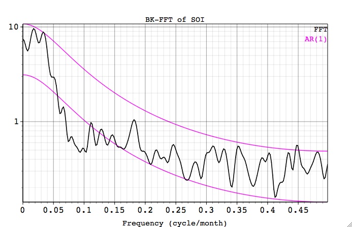
The significance test against AR(1) process can not distinguish these low-frequency peaks from the red-noise process. Thus, we need to apply more sophisticated tools, i.e. SSA and MTM, to determine oscillatory origin of these peaks.
By selecting the Cross-Spectrum check box, user can choose another vector to compute cross-spectra with the Data vector. Both vectors should have the same length, and the cross-spectra will be computed based on the individual correlogram estimates with the specified Window type, size, and number of frequencies. Next figure shows the cross-spectra between the SOI time series, and its SSA-filtered version which includes only two significant low-frequency oscillatory modes.
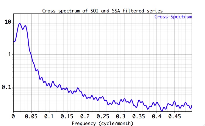
Most of the cross-spectrum's power is concentrated at the lower frequencies with two apparent peaks, compare it with the MTM Coherence estimate.
|
|
|