 |
 |
 |
(Note: In demo version MSSA Gap-Filling is available only for data in example projects. In a licensed copy this feature is enabled after activation with a purchased Serial No.)
A novel, iterative form of MSSA is used to analyze multivariate datasets with uneven sampling or missing observations. Gaps are filled-in by utilizing spatio-temporal correlations in the dataset. File data with "NaN" values (case insensitive) are treated as missing. Gap-filling feature is available in Advanced options of MSS/PCA panel. For univariate datasets pls. see SSA gap-filling.
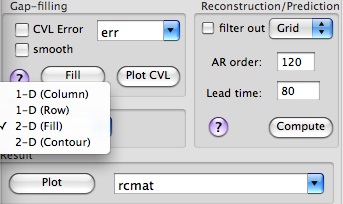
The user needs to select the data in the Data pop-up menu of MSSA/PCA tool, and then specify the PCA or MSSA method to fill the data. PCA will use only spatial correlations between the channels using a few leading EOFs up to the number specified on MSSA/PCA panel. MSSA, on the other hand, will in addition utilize temporal correlations as well; user needs to specify MSSA window size and the number of MSSA components for fill-in. Then gap-filling can be done just by clicking Fill in Gap-filling box of Advanced options.
The filled-in data is stored in the data with a name specified in Result box, while the MSSA/PCA spectral estimate is stored in matrix with a name specified in Spectrum box on main MSSA panel. Estimated leading ST-EOFs and T-PCs, up to the specified number of MSSA components, are stored in matrices with names obtained by prefixing "eof_", "steof_" and "pc_" to a Spectrum name, and can be accessed in Data I/O tool. They can be plotted by selecting rows from MSSA components table in Advanced options, setting a plot option, i.e. 1-D or 2-D (Fill or Contour) at the bottom of Advanced MSSA panel and hitting a Plot PCs or Plot EOFs button. The estimated leading ST-EOFs and T-PCs can be used for reconstruction as well.
By clicking Plot in Result, user can compare the gappy and filled-in dataset, if the column (spatial channel) or row (time channel) 1-D plot option has been selected. Alternatively, 2-D time-space plot can be created with Contour or Fill option.
When plotting missing data, user can select in Preferences option to connect all the available points through gaps:
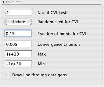
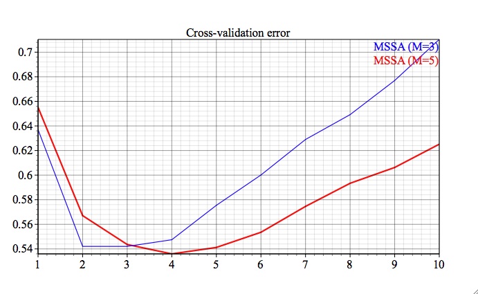
The number of MSSA components one has to use really depends on the dataset, and in particular on the amount of noise present. The main idea is to discard higher-ranked components corresponding to noise. If CVL error box is checked in Gap-filling options, a number of cross-validation experiments is performed (set in Preferences), where a small portion of the existing points is flagged as being missing (in random), and the rms error is calculated for filled-in data. The optimum number of components corresponds to a minimum of such error averaged over all cross-validation sets. The error can be plotted by Plot CVL button. The random seed for choosing the points for cross-validation can be changed in Preferences, as well as convergence criterion for missing values. User can perform such cross-validation experiments for different MSSA Window values in order to find optimum parameters for gap-filling. In addition, range of values of filled-in data can be constrained by setting optional Max and Min limits. The percentage of the dataset variance used to fill the gaps is written to Log. If results from several gap-filling calculations have been stored in different matrices, the parameters used (including Preferences) will be restored in GUI by simply selecting correspondent matrix from a Result pop-up list.
Here we demonstrate Toolkit capabilities for gap filling on synthetic time series following Examples/Multivariate Gap Filling folder of kSpectra distribution.
First, we will demonstrate MSSA and PCA gap filling of a noisy multivariate data containing quasi-periodic oscillatory spatio-temporal pattern. The synthetic test series, consisting of 20 spatial channels, each 100 data points long, represents low-frequency oscillation with a period of T=40 units. This oscillation is modulated both in amplitude and phase with period of T=120, and is contaminated by large amplitude white noise.
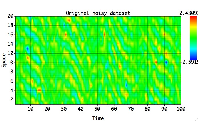
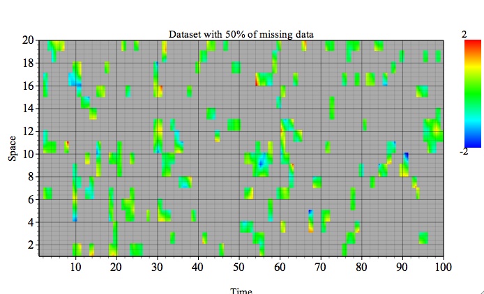
At a fixed time, the pattern represents standing wave in space. About 50% of the data there has been removed in random and filled-in with MSSA and PCA, and results are compared with the original (full) dataset:
Cross-validation shows which MSSA/PCA parameters are best for gap-filling:
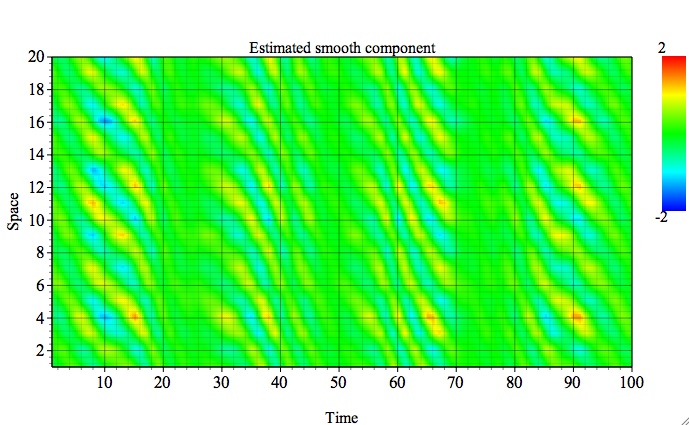
If smooth box is checked in Gap-filling options, then Result will be the estimated smooth component of dataset in all points, including those where data is available. Otherwise, Result will take values of existing data, and the missing values will be filled-in with the smooth component. So we check smooth box, and with MSSAWindow equal to 5, `BK' Covariance and 4 MSSA Components we obtain:
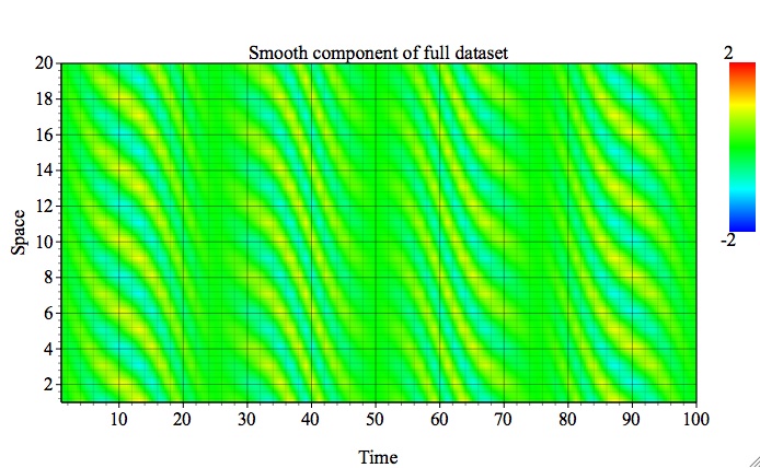
This result can be compared with a 'true smooth' component from the full dataset:
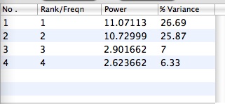
Log or/and MSSA components table in Advanced options shows that leading four MSSA components captured ~65% of the dataset variance that has been used to fill the gaps:
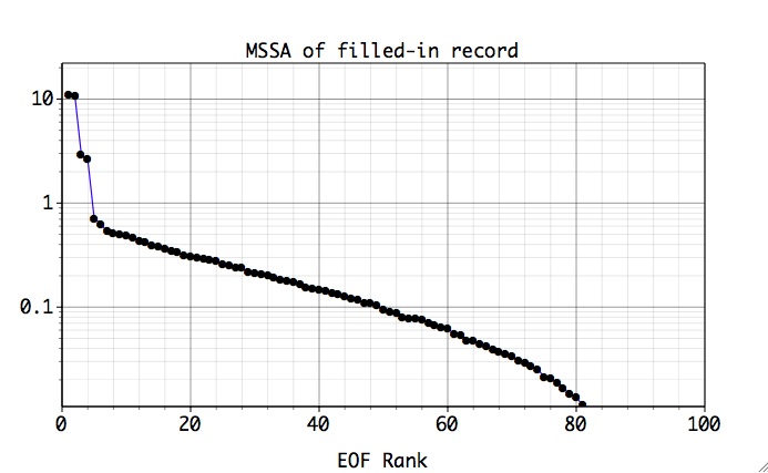
On main MSSA panel click Plot to see MSSA spectral estimate of filled-in data. Sharp break in the slop indicates separation of four leading oscillatory modes that have been used for gap-filling.
|
|
|
|