
 |
 |
 |
The basic idea is the same as in SSA prediction for univariate data. Prediction is started by performing MSSA filtering on input multivariate time-series to identify "signal" components, i.e. containing quasi-oscillatory modes and/or trend. Next, we fit AR model to "signal" PCs and advance them in time to produce PCs forecasts. Finally, MSSA reconstruction is performed that takes into account PCs forecasts. For small order of AR model, forecast errors are dominated by the lack of resolution; for large order, by the error made on the coefficients of the model.
Here we demonstrate MSSA prediction on synthetic data with two time series following prediction.tkt project in Examples/MSSA Prediction folder of kSpectra distribution. The 1st channel of our test series, 600 data points long, contains sinusoidal oscillation, modulated in amplitude and contaminated by noise. The 2nd channel consists of a similar but phase-shifted oscillation without noise; the 2nd channel can be considered as a "driver", while the 1st being a "response", or vice-versa:
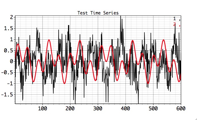
Our task will be to predict smooth signal in both channels 200 sampling units ahead, i.e. with 200 lead time. Unlike SSA prediction, forecast for multivariate data is driven by cross-channel temporal correlations.
We start kSpectra, and go to Data I/O in Tools. Using Finder, we simply double-click prediction.tkt file in MSSA Prediction folder. It contains datam1 (original data as above). Then we go to PCA/MSSA in Tools, select datam1 from Data Pop-up menu, change the Window value to M=300 (half of the time series length for better MSSA resolution), select Reduced method for Covariance, MSSA tool option, and set name in Spectrum box to mssa. Then click Compute, followed by Plot, to obtain MSSA spectral estimate:
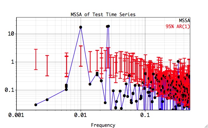
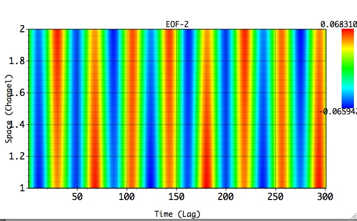
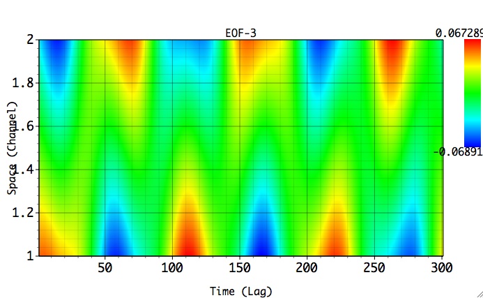
Low-frequency part of the spectrum contains two oscillatory EOF pairs which correspond to smooth quasi-periodic signal in both channels. These pairs can be inspected visually by opening Advanced panel, selecting 2nd and 3rd r rows in MSSA Components table, and using Plot EOFs with 2-D Fill plot option. We can readily see that this dataset is dominated by in-phase and out-of-phase oscillatory components.
Now select leading four rows of MSSA components table corresponding to oscillatory pairs of the signal, and set Lead time to 200, AR order to 300 in Prediction/Reconstruction box, and then click Compute.
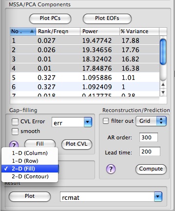
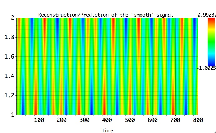
To see 2-D plot of Reconstructed & Predicted "smooth" signal in both channels, choose 2-D Fill Plot option as above, and click Plot in Result to obtain Figure below:
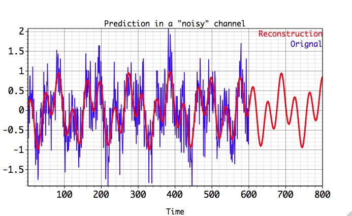
To plot Reconstructed & Predicted "smooth" signal with original data in a single channel, choose 1-D (Column) Plot option, 1st column, and then click Plot in Result to obtain Figure below:
|
|
|
|