
 |
 |
 |
As an example, we apply MSSA to the near-global data set of monthly sea-surface temperatures (SSTs) anomalies data set for 1950-2004, from 30° S to 60° N, on a 10° latitude x 10° longitude grid (International Research Institute for Climate and Society (IRI), see sst_mssa.tkt project in Examples/Oceanography folder)
This translates into a dataset with 360 channels (36 longitude x10 latitude), 648 months long. The channels with NaN values in all rows indicate land mask, and there are 247 channels with actual data. The input data is a matrix with a name "sst", which has 648 rows (time-coordinate) and 360 columns (space coordinate). To setup a 2-D grid for display of the spatial coordinate, we factor number of columns (cols) and set col1 and col2 values for sst matrix as 36 and 10, respectively.
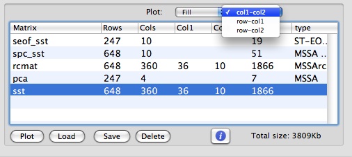
Then, all relevant MSSA (PCA) results for this matrix will be obtained and can plotted using 2-D grid for spatial coordinate. For Fill or Contour 2-D plots, such dataset can be plotted in col1-col2, row-col1 and row-col2 coordinates. For Fill and col1-col2 options we obtain the following plot:
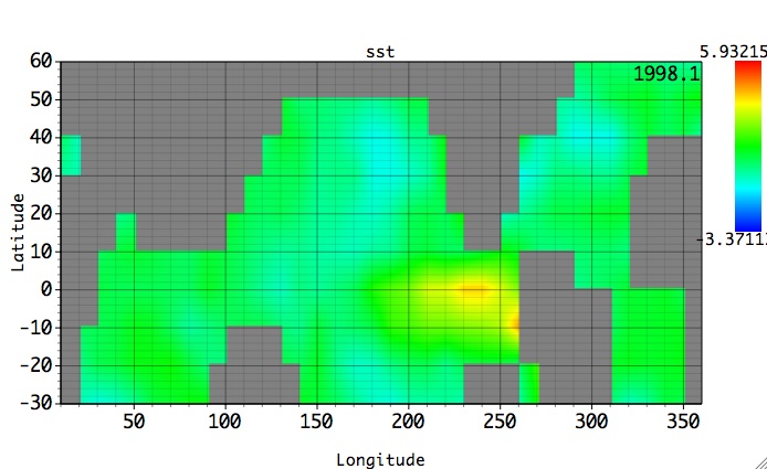
Then we can browse through the 3rd dimension of this dataset -- row (time), by using Graph Controls/Axes/2D option:
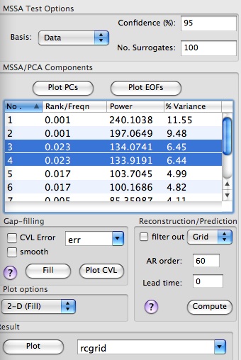
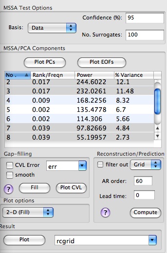
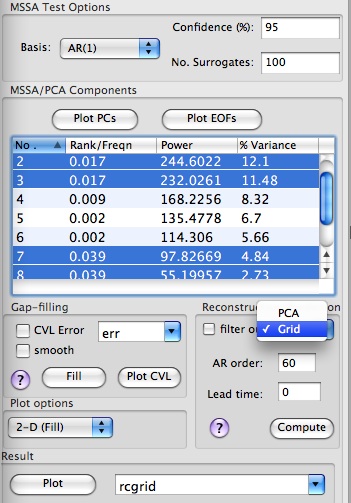
Selecting the `MSSA/PCA' option from the Tools menu on the main panel launches the following window:
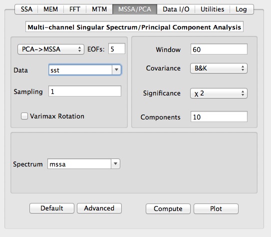
Having selected the data to be analyzed (here `sst') and the sampling interval, user can choose analysis type, i.e. PCA, MSSA or PCA->MSSA, which is MSSA done on data compressed by PCA.
Main options for MSSA are temporal Window Length, type of Significance
Test, Covariance method, and number of spatial EOFs channels (for PCA->MSSA). The number of Components specifies how many MSSA components will be retained for Reconstruction/Prediction. Results of PCA/MSSA are stored in matrix with a name specified in Spectrum field. In addition, T-EOFs, ST-EOFs and T-PCs are stored in matrices with names obtained by prefixing "eof_", "steof_" and "pc_" to a Spectrum name, and can be accessed in Data I/O tool.
If results from several analyses have been stored in different matrices, the parameters used in a particular computation will be restored in GUI by simply selecting correspondent matrix from a Spectrum pop-up list. Get Default Values button is provided as a guide.
In general, it is better to choose the Reduced Covariance estimator for data with many spatial channels L and large temporal window M, so when ML > N' it is more efficient to diagonalize the reduced N' x N' covariance matrix, rather than the LM x LM
Varimax Rotation has been introudced initiallyfor better physical interpretation of EOFs from PCA. Recently, Groth and Ghil (2011) have demonstrated that a classical M-SSA analysis suffers from a degeneracy problem, with eigenvectors not well separating between distinct oscillations when the corresponding eigenvalues are similar in size. This problem is a shortcoming of principal component analysis in general, not just of M-SSA in particular. In order to reduce mixture effects and to improve the physical interpretation, Groth and Ghil (2011) have proposed a subsequent varimax rotation of the ST-EOFs. To avoid a loss of spectral properties (Plaut and Vautard 1994), they have introduced a slight modification of the common varimax rotation that takes the spatio-temporal structure of ST-EOFs into account.
Varimax rotation is applied to leading number of MSSA or PCA components specified in Components field if the Varimax Rotation box is checked. MSSA with Varimax Rotation is demonstrated on Multivariate Small Signal example.
For the example below we don't apply varimax rotation so we leave the box unchecked as above.
To demonstrate the usage of N'-windows vs. M-windows, we will use `Reduced' and `Broomhead &King` options. For `Broomhead &King`, we will set the Window to 60, corresponding to 5 years. For Reduced option we will set the Window to 324, which provides maximum spectral resolution (M=N'=N/2).
Choosing Chi-squared in the Significance tests menu, for `Reduced` covariance and M=N'=324 we obtain the following plot:
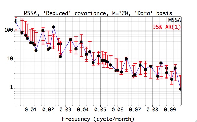
Here the data and red-noise error bars are plotted against the dominant frequencies associated with each MSSA mode. The dominant frequencies of MSSA modes are computed only for the Monte-Carlo or approximate, but much faster, Chi-squared test. The frequencies and variances captured by each mode are displayed in a components table of Advanced options panel. For M=N'=324 and 'Reduced' covariance, the significant oscillatory quasi-quadrennial pair formed by modes 3 and 4, captures only 13.1% of variance of our input data (5 leading PCs from PCA):
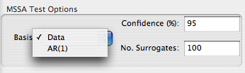
The quasi-biennial pair (modes 13 and 14) does not pass the significance test when data eigenmodes are used as a basis for projections. However since the Monte-Carlo test is biased if we project onto the data eigenmodes, we will use the eigenmodes provided by the covariance matrix of the AR(1) process. So, we select AR(1) instead of Data basis in MSSA Test Options of Advanced Options panel:
, and repeat computation to obtain the following result:
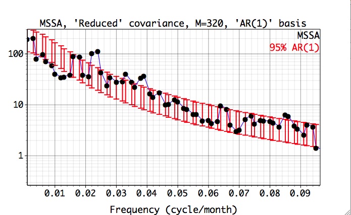
Here, the projections are plotted against the dominant frequencies associated with each noise eigenvector, and we have zoomed in on the 0-0.07 cy/month frequency interval of interest. Since the latter are near-sinusoidal in this case, the resulting spectrum is closely related to a traditional Fourier power spectrum. Both the quasi-quadrennial(~0.023 cycle/month) and the quasi-biennial(~0.033 cycle/month) modes pass the test at the 95% level (as specified in Test Options). They are well separated in frequency by about 1/(20 months), which far exceeds the maximum spectral resolution of 1/M = 1/N' =1/324 months.
It is useful to verify the above results with the Monte-Carlo test, using randomly generated red-noise surrogates. For large datasets such computation may take a long time.
In contrast to `Reduced` covariance, when using `Broomhead &King` option and M=60, both the quasi-quadrennial (modes 2 and 3 in this case) and quasi-biennial (mode 7 and 8) pairs appear to be well resolved and significant:
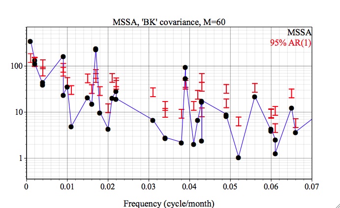
The quasi-quadrennial pair accounts ~ 23% of variance of input data, while less energetic quasi-biennial accounts for ~ 7%.
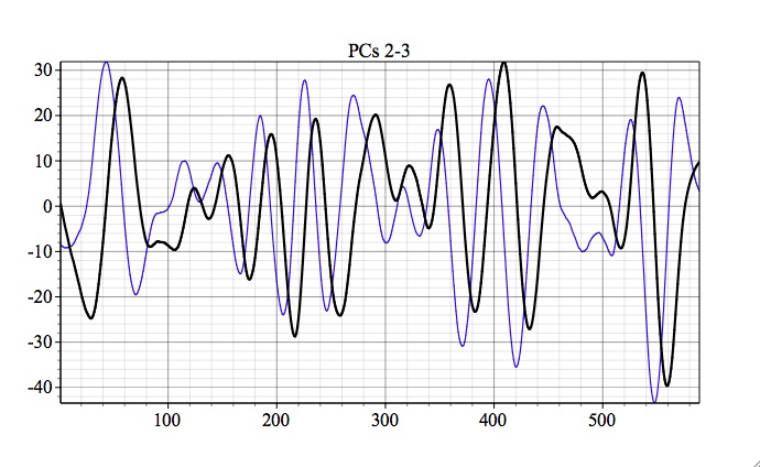
We can check whether a pair of selected MSSA modes are indeed in phase quadrature and form oscillatory pair, by plotting their PCs, and/or inspecting their EOFs. We can do so by selecting rows from MSSA components table, setting a plot option, i.e. 1-D or 2-D (Fill or Contour) at the bottom of Advanced MSSA panel and hitting a Plot PCs or Plot EOFs button.
The following plot is for the EOF of 2nd MSSA component (`Broomhead &King` option and M=60) using 2-D Fill plot option:
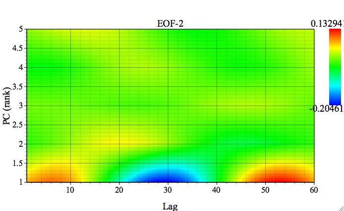
This plot shows how a single MSSA EOF is expressed in all of the channels of input data (here 5 components of PCA). As one can see, it is prominent mainly in the 1st channel of input data, with a clear oscillatory behavior. Alternatively, one can compare different EOFs in a single channel by using 1-D Plot option:

We can see that the 3rd mode is mostly energetic in the 1st channel as well, by selecting 2nd and 3rd row of MSSA components table, setting Plot Options as above and hit Plot EOFs button:
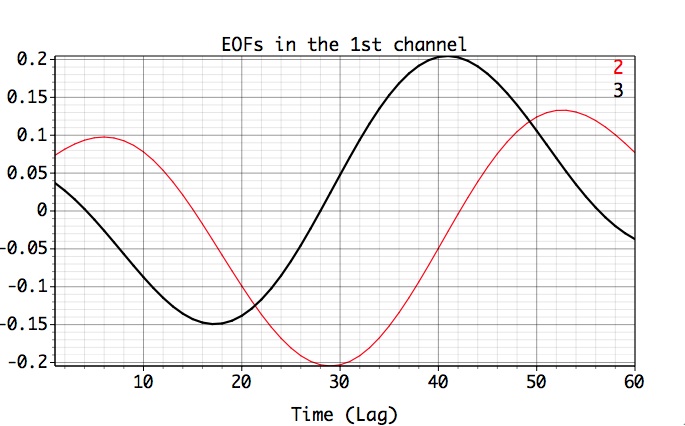
The associated PCs are also in phase quadrature, as expected:
For overview of prediction Options (AR order and Lead) see MSSA prediction.
We can reconstruct contributions from selected MSSA components in Components table of Advanced panel in original Grid or PCA space ,by choosing Grid or PCA in Reconstruction box:
The name of matrix with reconstruction is specified by the user in Result box at the bottom of Advanced options panel. By clicking Plot, user can compare reconstruction vs. original data in a specified channel, if 1-D plot option (column or row) is selected. The plot below shows contribution of oscillatory pairs in the leading PC from the PCA, using 1-D plot and PCA reconstruction options:
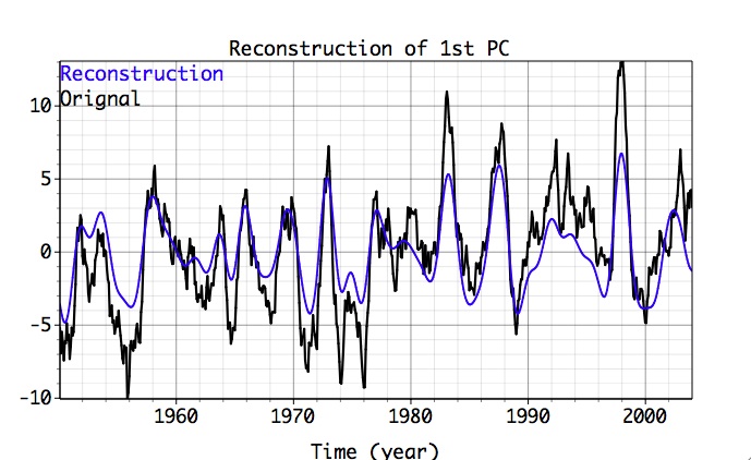
If 2-D Plot option is chosen (Contour or Fill), reconstructed data only will be plotted in 2-D time-space coordinates; the figure below shows contribution of the oscillatory pairs in all input PCs from PCA, using 1-D plot and PCA reconstruction options:
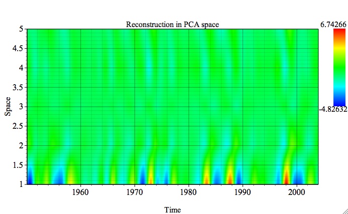
The figure below shows reconstruction of original gridded data (Grid option), displayed with a 2-D Fill plot option. Since the spatial dimension of gridded input data has been 2-D factored (i.e x*y or col1*col2) using col1 and col2 in Data I/O Matrices table, the plot will be displayed also in x-y:
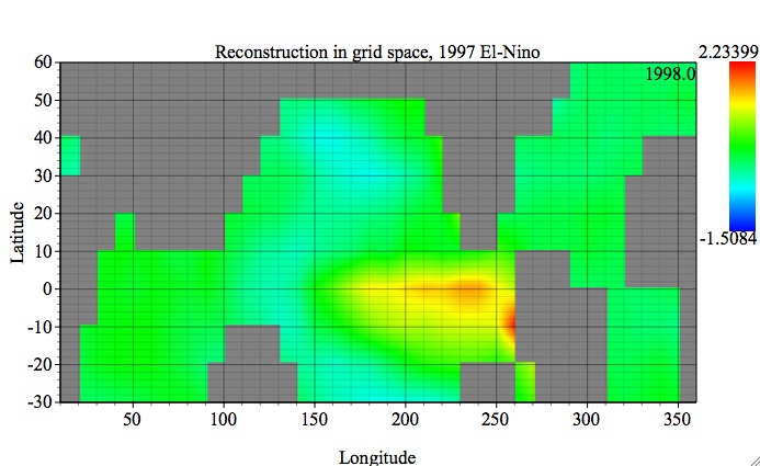
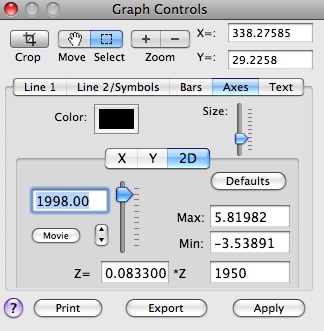
Then we can browse through the Z dimension of this dataset -- time, by using slider, stepper or text field in Graph Controls/Axes/2D:
The Movie button makes a QuickTime movie animation of the 2-D Active Plot along the dataset's Z dimension (here time) and exports it to a file using Save As panel.
Linear transformation can be applied to the Z dimension of 2D plots in Axes/2D settings. Parameters of the transformation has to be set first. To return to the default settings, use transformation factors 1.0 and 0.0 (as in Z=1*Z + 0), or Defaults button. Above panels show how the transformation is applied to have time in calendar years, instead of months. User can also adjust the Max and Min values of the plotted field in Graph Controls/Axes/2D.
|
|
|
|